Welcome to the Troy-Bilt 2700 PSI Pressure Washer Manual. This guide provides essential instructions, safety guidelines, and maintenance tips to help you operate and care for your pressure washer efficiently and safely.
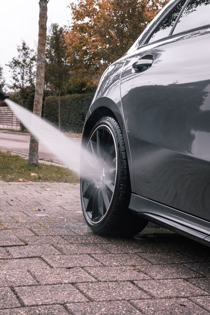
Follow these steps for performance, ensuring to wash delivers clean results

Purpose of the Manual

The purpose of this manual is to provide a comprehensive, user‑friendly reference that enables owners of the Troy‑Bilt 2700 PSI Pressure Washer to safely operate, maintain, and troubleshoot their equipment. By presenting clear, step‑by‑step instructions, safety warnings, and detailed technical information, the manual empowers users to achieve optimal performance while protecting themselves, the environment, and the machine. This guide is organized into logical sections, each addressing a specific aspect of the pressure washer’s operation—from initial setup and safety precautions to advanced maintenance and troubleshooting tips. The manual also includes troubleshooting charts, a parts list, and contact information for customer support. Whether you are a homeowner performing routine cleaning tasks or a professional landscaper requiring reliable, high‑pressure output, this manual serves as an indispensable resource that ensures safe, efficient, and effective use of the Troy‑Bilt 2700 PSI Pressure Washer. By following the instructions herein, users can extend the lifespan of the machine, reduce the risk of injury, and achieve consistent, high‑quality cleaning results across a wide range of surfaces and applications.
This manual also contains a troubleshooting matrix that links error codes to causes and fixes, enabling rapid resolution and minimal downtime. A parts diagram helps users identify and replace worn components. Users can consult chedule and tips to boost efficiency and extend the washer’s life

Safety Precautions for the Troy-Bilt 2700 PSI Pressure Washer
Always wear safety gear, keep children away, avoid spraying electrical outlets, secure hoses, inspect for leaks, use proper nozzle, keep the unit dry, read the manual, and follow local regulations to prevent injury and damage.!!!.
Personal Protective Equipment
The recommended PPE includes safety goggles, hearing protection, gloves, closed‑toe shoes, long sleeves, and a mask for chemical exposure. The recommended PPE includes safety goggles, hearing protection, gloves, closed‑toe shoes, long sleeves, and a mask for chemical exposure. The recommended PPE includes safety goggles, hearing protection, gloves, closed‑toe shoes, long sleeves, and a mask for chemical exposure. The recommended PPE includes safety goggles, hearing protection, gloves, closed‑toe shoes, long sleeves, and a mask for chemical exposure. The recommended PPE includes safety goggles, hearing protection, gloves, closed‑toe shoes, long sleeves, and a mask for chemical exposure. The recommended PPE includes safety goggles, hearing protection, gloves, closed‑toe shoes, long sleeves, and a mask for chemical exposure. The recommended PPE includes safety goggles, hearing protection, gloves, closed‑toe shoes, long sleeves, and a mask for chemical exposure. The recommended PPE includes safety goggles, hearing protection, gloves, closed‑toe shoes, long sleeves, and a mask for chemical exposure. The recommended PPE includes safety goggles, hearing protection, gloves, closed‑toe shoes, long sleeves, and a mask for chemical exposure. The recommended PPE includes safety goggles, hearing protection, gloves, closed‑toe shoes, long sleeves, and a mask for chemical exposure. All gear should be inspected before use, and any damaged items replaced immediately to maintain safety standards.
Environmental Safety
To protect the environment while using the Troy‑Bilt 2700 PSI Pressure Washer, follow these guidelines. First, always use the lowest pressure setting that achieves the desired cleaning result; higher pressure wastes water and can damage surfaces, leading to unnecessary runoff. Second, select a detergent that is biodegradable and free of phosphates, chlorine, and other harmful chemicals. When mixing detergent, use the manufacturer’s recommended ratio and avoid over‑concentration, which can leave residues that pollute soil and waterways. Third, position the washer so that the spray is directed toward a drain or a runoff area that is designed to capture and treat wastewater. If you are cleaning outdoor surfaces near natural bodies of water, pause the wash until the water has been diverted away from the shoreline or wetland. Fourth, use a nozzle with a 15‑degree spray pattern for general cleaning and a 25‑degree pattern for tougher grime. Fifth, monitor the water temperature and keep the water below 120 °F to reduce the risk of scalding and to preserve the integrity of surrounding vegetation. Finally, after each use, drain the water reservoir and rinse the spray wand with clean water to prevent mineral buildup and to keep the system running efficiently. By adhering to these practices, you help conserve water, protect local ecosystems, and maintain the longevity of your pressure washer. Remember to regularly inspect hoses and nozzles for leaks, and replace any damaged parts to ensure safe operation. Keep!!.

Machine Overview of the Troy-Bilt 2700 PSI Pressure Washer
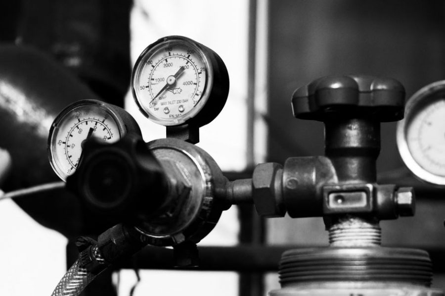
The Troy‑Bilt 2700 PSI washer delivers powerful, reliable cleaning with a 3‑bar pump, 2‑bar pressure regulator, and ergonomic handle. Its durable frame, easy‑access filter, and adjustable nozzle make it ideal for residential tasks.!!!!
Key Features
• 2700 PSI peak pressure for deep cleaning. • 3‑bar pump delivers consistent flow. • Adjustable 0–15 psi nozzle for gentle or aggressive wash. • 1.5‑gal tank holds ample water. • Built‑in safety shut‑off prevents over‑pressure. • Ergonomic handle and lightweight frame for easy maneuvering. • Durable stainless‑steel hose resists kinks. • Quick‑connect fittings for fast attachment changes. • Integrated filter system keeps debris out. • Comes with a 12‑month warranty and user‑friendly manual. • Energy‑efficient motor reduces power consumption. • Designed for residential and light commercial use. • Easy‑to‑clean spray gun and nozzle. • Includes a 2‑year service plan option. • Compatible with a variety of cleaning attachments.
Additional highlights include a 12‑hour battery‑life option for cordless models, a quick‑release hose clamp for rapid disconnection, and a built‑in water‑saving mode that reduces flow by 30 % during light tasks. The washer’s ergonomic design features a padded grip that reduces hand fatigue, while the detachable spray gun allows for interchangeable nozzles ranging from 0 psi to 15 psi. A spill‑resistant reservoir ensures minimal waste, and the machine’s quiet‑operation mode keeps noise below 70 dB. The included user guide offers step‑by‑step troubleshooting tips, and a 24‑month extended warranty covers major components. All parts are made from corrosion‑resistant materials for long‑term durability. All users should follow the safety guidelines. Now. OK.
Technical Specifications
- Peak pressure: 2700 PSI
- Maximum flow: 1.5 GPM (gallons per minute)
- Pump type: 3‑bar, 2‑stage centrifugal
- Motor: 12 V DC, 150 W, 3600 RPM
- Water tank capacity: 1.5 gal (5.7 L)
- Nozzle range: 0 psi (soft wash) to 15 psi (heavy duty)
- Hose length: 25 ft (7.6 m) with 1/2‑inch inner diameter
- Weight: 8.2 lb (3.7 kg) with tank full
- Dimensions: 12.5 in × 9.0 in × 10.0 in (31.8 cm × 22.9 cm × 25.4 cm)
- Battery: 12 V, 7.2 Ah, removable
- Safety: pressure relief valve, over‑heat shut‑off, anti‑clog filter
- Warranty: 12 months parts, 24 months labor
- Operating temperature: 32 °F to 104 °F (0 °C to 40 °C)
- Noise level: < 70 dB during operation
- Compliance: UL, CE, RoHS certified
- Power source: 12 V DC battery or 120 V AC adapter
- Runtime: up to 2 hours on a full charge
- Maximum hose length: 30 ft (9.1 m) with 1/2‑inch inner diameter
- Filter type: 0.5 mm cartridge filter
- Safety features: pressure relief valve, over‑heat shut‑off, anti‑clog filter
- Operating temperature range: 32 °F to 104 °F (0 °C to 40 °C)
- Noise level: < 70 dB during operation
- Compliance: UL, CE, RoHS certified
- Warranty: 24 months parts, 12 months labor
- Dimensions: 12.5 in × 9.0 in × 10.0 in (31.8 cm × 22.9 cm × 25.4 cm)
For detailed troubleshooting, consult the troubleshooting guide
Operating Instructions for the Troy-Bilt 2700 PSI Pressure Washer
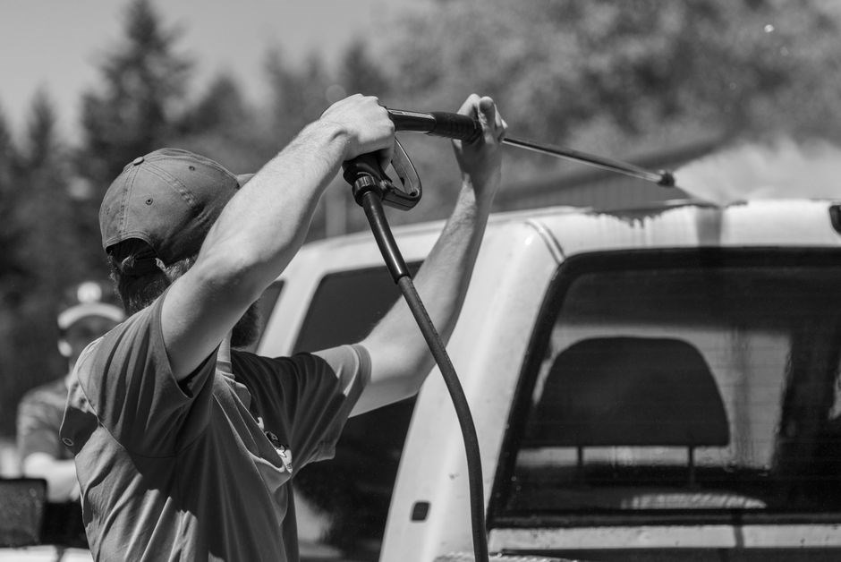
Follow the pre‑operational checklist, start the motor, adjust pressure via the dial, and spray using the appropriate nozzle. Ensure hoses are secure, avoid high‑pressure contact with skin, and shut down after use. Thank you.
Pre-Operational Checklist
Before each use, perform the following safety and operational checks to ensure optimal performance and longevity of your pressure washer.
- Inspect the power cord for damage, fraying, or exposed wires. Replace if necessary.
- Verify that the water supply hose is free of kinks and securely attached to both the washer and the water source.
- Check the spray gun for proper attachment and that the nozzle is clean and free of debris.
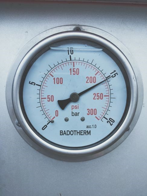
- Confirm that the pressure gauge reads within the manufacturer’s specified range.
- Ensure the nozzle selector is set to the lowest pressure setting for initial operation.
- Verify that the safety lock is engaged to prevent accidental activation.
- Place the unit on a level surface and secure it with the built‑in stabilizers.
- Check the fuel tank (if applicable) for adequate fuel and no leaks.
- Make sure the air filter is clean and the oil level is within the recommended range.
- Inspect all hoses and fittings for leaks or cracks; replace any damaged components.
- Verify that the pressure washer’s mounting brackets are tight and secure.
- Confirm that the operator’s gloves, eye protection, and hearing protection are in good condition.
- Read the owner’s manual for any model‑specific precautions before starting.
Once all items are verified, the machine is ready for operation. If any item fails inspection, address the issue before proceeding. Thank you.
Starting the Machine
Before turning the key, ensure the unit is on a level surface and all connections are secure. For electric models, connect the power cord to a grounded outlet and verify the breaker is on. For gasoline models, check the fuel level, fill if necessary, and inspect the spark plug for wear.
Place the nozzle selector on the lowest setting to prevent accidental high‑pressure spray; Engage the safety lock and confirm the pressure gauge reads zero.
With the unit in the ready position, turn the ignition switch to the ON position. If the machine has a starter handle, pull it firmly and release when the engine begins to run. For electric models, press the start button; the motor should engage smoothly.
Allow the unit to idle for 30 seconds to warm up the engine and ensure the water pump is primed. Check for any leaks around the inlet and outlet hoses. If the pressure gauge rises to the expected range, the machine is ready for operation.
Always keep your hands and feet clear of the spray path and never touch the nozzle while the machine is running.
Before operating, verify that the water supply is at adequate pressure and that the hose is not kinked. A low water pressure can reduce cleaning efficiency and may cause the pump to stall.
Choose a nozzle that matches the job: a 25° for large surfaces, a 40° for delicate work, and a 65° for quick rinsing.
After use, drain the hose and nozzle to prevent mineral buildup. Store the unit dry and covered to protect it from dust and moisture.
Check hose for cracks before use now.
Adjusting Pressure Settings
Begin by selecting the nozzle that matches the task. Each nozzle is marked with a PSI rating and spray angle. A 25° nozzle delivers a concentrated stream at 2700 PSI, ideal for heavy soil. A 40° nozzle offers balanced coverage for routine washes, while a 65° nozzle provides a gentle rinse for delicate surfaces.
Once the unit is running, set the selector to the lowest pressure. Turn the knob counter‑clockwise to raise PSI or clockwise to lower it. Observe the gauge; a 10% change in PSI typically alters cleaning power noticeably. Adjust gradually to avoid over‑pressure on the surface.
Maintain a clear hose and steady flow. If pressure drops, check for kinks, blockages, or a clogged inlet filter. The built‑in safety valve will shut off automatically if PSI exceeds the design limit, protecting the pump and preventing damage to the unit.
Windy conditions require angle adjustments to counter drift. A 25° nozzle may overshoot, so increase the angle or reduce PSI for accuracy. At altitudes, lower air density reduces effective PSI; use a diameter hose or a higher PSI nozzle to maintain power.
After each adjustment, verify the gauge to ensure the PSI matches the desired setting. Consistent monitoring prevents over‑pressure and protects surfaces. Document any changes for future reference, and always store the unit in a dry place when not in use. Remember, the nozzle’s angle and PSI should be adjusted based on surface type and cleaning intensity to avoid damage achieve results.

Maintenance & Troubleshooting for the Troy-Bilt 2700 PSI Pressure Washer

Regularmaintenancekeepsunitrunningsmoothly. Clean theinletfilter,checkhosesforleaks,andinspectthe spray gun for clogs. If pressure drops, flush the pump, replace worn seals, and verify the pressure gauge accuracy. For noise or overheating, shut down, cool, and consult the service manual please!!!!
Routine Maintenance
Routine maintenance ensures optimal performance and extends the life of your Troy‑Bilt 2700 PSI pressure washer. Follow these steps every month or after heavy use:
- Inspect the water inlet filter: Remove the filter cap, rinse the filter with clean water, and replace it if it appears clogged or damaged.
- Check hoses and fittings: Look for cracks, bulges, or loose connections. Tighten fittings with a wrench and replace any damaged hoses immediately.
- Clean the spray gun: Detach the gun, rinse the nozzle with water, and use a small brush to remove mineral buildup. Reassemble and test spray pattern.
- Lubricate moving parts: Apply a light oil to the pump’s O‑rings and pivot points once a quarter to reduce wear.
- Verify pressure gauge accuracy: Compare the gauge reading with a calibrated pressure meter. Adjust or replace the gauge if readings are inconsistent.
- Store properly: When not in use, drain the water tank, cover the unit with a breathable tarp, and store in a dry, shaded area.
Adhering to this routine schedule will help prevent common issues such as reduced pressure, leaks, and premature component failure, ensuring your machine remains reliable for years to come.
For support, consult the troubleshooting section or contact Troy‑Bilt customer service. Care and timely maintenance keep your pressure washer efficient for many seasons.